Breaking Neural Networks, Part 1 — Turning A Frog Into A Cat
We’ve all seen the hype. Deep Learning techniques can recognize human faces in a crowd, identify seals from orbit, and classify insects from your phone! SkyNet awaits!
Well, not today, everybody. Because today is the day we fight back. But we won’t be sending back John Connor to save the day. Oh no, we’ll be using maths.
Okay, so first, we need a neural network to attack. Today, we’re not going to be sophisticated - we’re simply going to take an architecture from one of the PyTorch tutorials. It’s a very shallow ConvNet for classifying images from the CIFAR-10 dataset, but the principles here scale up to something like Inception. We train the model, again just using the training code in the tutorial, and we begin.
What is this, oh clever neural network?
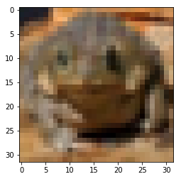
Model says: Frog
(CIFAR-10 images are only 32x32 pixels, so yes, it’s a touch blocky)
What we’re going to do is change our picture of a frog just enough that the neural network gets confused and thinks it’s something else, even though we can still recognize that it’s clearly a frog, thus proving man’s continued domination over machine.
To do this, we’re going to use a method of attack called the fast gradient sign method, which was detailed back in 2014 in this paper by Ian Goodfellow , Jonathon Shlens & Christian Szegedy.
The idea is that we take the image we want to mis-classify and run it through the model as normal, which gives us an output tensor. Normally for predictions, we’d look to see which of the tensor’s values was the highest and use that as the index into our classes. But this time, we’re going to pretend that we’re training the network again and backpropagate that result back through the model, giving us the gradient changes of the model with respect to the original input (in this case, our picture of a frog).
Having done that, we create a new tensor that looks at these gradients and replaces an entry with +1 if the gradient is positive and -1 if the gradient is negative. That gives us the direction of travel that this image is pushing the model. We then multiply by a scalar, epsilion to produce our malicious mask, which we then add to the original image, creating an adversarial example.
Here’s a simple PyTorch method that returns the fast gradient sign tensors for a input batch when supplied with the batch’s labels, plus the model and the loss function used to evaluate the model:
    def fgsm(input_tensor, labels, epsilon=0.02, loss_function, model):
        outputs = model(input_tensor)
        loss = loss_function(outputs, labels)
        loss.backward(retain_variables=True)
        fsgm = torch.sign(inputs.grad) * epsilon
        return fgsm
(epsilon is normally found via experimentation - 0.02 works good for this model, but you could also use something like grid search to find the value that turns a frog into a ship)
Running this function on our frog and our model, we get a mask that looks like this:
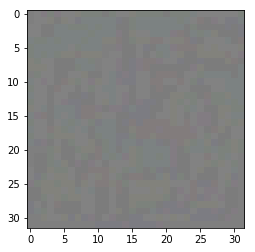
Adding that mask to the frog results in:
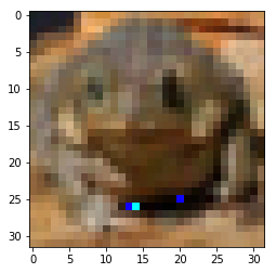
Clearly, still a frog. What does our model say?
model.predict() -> "cat"
Hurrah! We have defeated the computer! Victory!
Eagle-eyed readers will have noticed that in order to produce an image that fools the classifier, we need to know a lot about the model being used. We need the explicit outputs so we can run backpropagation to get our gradients, and we need to know the actual loss function the model uses to make this work. This is fine for this example, because we know everything about the model, but if we wanted to fool a classifier where we don’t have access to any of these internals, we’re stuck. Right?
Stand by for Part 2 soon, where we discover how we can extend this approach to defeat classifiers where all we get is ‘this is a frog’. We shall defeat the machines!