Image Self-Supervised Training With PyTorch Lightning
May 25, 2020 · 13 minute read(You can also view this post in Google Colab)
Self-Supervision is the current hotness of deep learning. Yes, deep networks and transfer learning are now old hat — you need to include self-supervised somewhere if you want to get those big VC dollars. Like transfer learning, though at its core it’s a very simple idea: there is so much data in the world — how can we use it without the big expense of getting humans to label it all? And the answer really does feel like cheating. Self-supervision is essentially “get the computer to automatically add labels to all your data, train a network on that, and then use transfer learning on the task you actually want to solve.” That’s it. The only interesting bits are how to decide what labels you add to what is called the “pretext task”, but the technique is surprisingly effective, especially in image and text-based problems where the Internet provides an almost endless supply of data.
Let’s have a look at the two main approaches to image self-supervised learning that are popular right now — rebuilding the original input from a distorted input, and automatically adding labels to data and training using those synthetic labels
Reconstructing & Augmenting The Input
If you remember our look at the super-resolution architectures, they’re taking a small image and producing a larger, enhanced image. A self-supervised dataset for this problem can be fairly easily obtained by simply looking at the problem in the opposite way: harvest images from the Internet, and create smaller versions of them. You now have training images and the ground truth labels (the original images). If you’re building a model that colourizes images, then you grab colour images…and turn them into black and white ones!
You can extend this to a more general principle, where you take an image, apply a series of transforms to that image, and then train a neural network to go from the manipulated image to the original. You’ll end up with some sort of U-Net-like architecture, but after you’ve trained the network, you can throw away the ‘decoder`’ half and use the ‘encoder’ part for your actual task by adding a Linear layer or two on top of the features you obtain at the bottom of the ‘U’.
You’ll want an augmentation technique that forces the architecture to learn things like how to structure elements of images, how to in-paint missing parts of an image, correct orientations, and so on. Here’s a couple to get you started
CutOut / Random Erasing
Perhaps the easiest to apply is simply removing part of an image and getting the model to restore it. This approach is often known as CutOut, and was shown to improve model performance with classification tasks in its introductory paper “Improved Regularization of Convolutional Neural Networks with Cutout”.
And it’s rather easy to apply, because it’s now included as a torchvision transform by default! You can just use:
torchvision.transforms.RandomErasing(p, scale, ratio value, inplace)
This can be slotted into a transform pipeline as we’ve seen many times throughout the book. The parameters you can set are:
p— the probability of the transform taking placescale— range of proportion of erased area against input image.ratio— range of aspect ratio of erased area.value— the value that will be used in the erased box. Default is 0. If given a single integer, that integer will be used. A tuple of length 3 will make the transform use values within for replacing R, G, and B channels. If passed the string"random", each pixel in the box will be replaced with a random value.inplace— boolean to make this transform inplace. Default set to False.
In general, you’ll probably want to use the random strategy for erasing details from an image.
Crappify
Crappify is a fun idea from the fast.ai project which literally ‘crappifies’ your images. The concept is simple: pack a transform function with resizing, adding text, and JPEG artefacting, or anything else you decide to add to ruin the image, and then train the network to restore things back to the original.
Automatically Labelling Data
The full image-based based self-supervision works very well, but you could say that it’s a little wasteful in a classification task; you end up training a full U-Net and throwing half of it away. Is there a way we can we be lazier and still do self-supervision?
Yes! And it’s what we’re going to spend the rest of this section implementing. Consider this image:

Okay, so it’s another picture of Helvetica the cat, but we would need a human annotator to give us the cat label. But we can take this image, transform it, and give it a meaningful label at the same time.
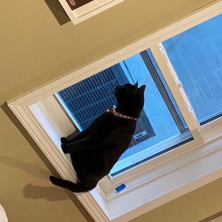
image_90
We have given this new image the label of image_90 to indicate that it has been indicated by 90º. But no human was needed in this (trivial) labelling. We can build a completely synthetic classification task, where we can build a training dataset and corresponding labels entirely programatically. We don’t need to build a U-Net block because all we’re training is a simple classification task; there’s no image reconstruction. But in order to learn how to classify correctly, the model will have to learn how to recognize what way up a cat normally is, and this pre-trained model can then be used on our actual classification task.
We’re going to build this approach to self-supervision, but we’re going to do it with a slightly higher-level framework than PyTorch. Enter PyTorch Lightning!
PyTorch Lightning, or A Little Help From The Internet
PyTorch Lightning is a wrapper around PyTorch that handles a lot of the standard PyTorch boilerplate that you end up writing for every project (e.g. training, test, and validation loops, determining whether a model should be in eval or not, setting up data, and so on). Like fast.ai, it has an extensible callback system that allows you to hook custom code during almost any part of the training cycle, so you end up with most of the power of PyTorch, but without having to rewrite train() every time you start a new project. Instead, you end up just doing this to train a custom model:
from pytorch_lightning import Trainer

model = LightningModel()
trainer = Trainer(gpus=1, num_nodes=1)
trainer.fit(model)
Some people prefer working with pure PyTorch all the time, but I definitely see a lot of value in Lightning, as it does remove a lot of the error-prone tedium of writing training code while still remaining flexible enough for research purposes. I personally write most of my deep learning code either with Lightning or fast.ai (the new fast.ai2 library even has a tiered layer of APIs that allows you to delve deeper when you need to but still use their powerful higher-level abstractions for most of your work) rather than in raw PyTorch.
Don’t worry, though, because as we’ll see, building a model with PyTorch Lightning isn’t that much different than what we’ve been doing throughout the rest of the book. We just don’t need to worry about the training quite so much!
Light Leaves, ResNet Sees
In order to demonstrate self-supervised training, we’re going to use a smaller version of ImageNet called Imagenette. This dataset contains images from 10 classes of the larger set, and was constructed by Jeremy Howard as a way of being able to quickly test new ideas on a representative sample of ImageNet rather than having to spend a considerable amount of time training on the whole thing. We’ll be using the full-sized version for our model, which means a 300Mb download. Let’s declare our imports and download Imagenette.
!pip install pytorch-lightning
import torch
import torch.nn as nn
import torch.nn.functional as F
import torchvision
import pytorch_lightning as pl
from PIL import Image
from pathlib import Path
from torchvision import transforms
import torchvision.transforms.functional as TF
import random

!wget https://s3.amazonaws.com/fast-ai-imageclas/imagenette2-320.tgz
!tar xvzf imagenette2-320.tgz
A Self-Supervised Dataset, As A Treat
You, sobbing: “You can’t just point at a picture and call it a label!"
Me, an intellectual, pointing at a cat rotated ninety degrees: “Label."
Even though we’re using PyTorch Lightning, we’ll construct our datasets in the usual way with the Dataset class. When an image is requested from the dataset, we will either simply return a tensor version of the image with the label 0, or randomly apply a rotational transform through 90, 180, or 270 degrees, or flipping the image’s axis either horizontally or vertically. Each of these potential transforms has a separate label, giving us six potential labels for any image. Note that we’re not doing any normalization in this pipeline to keep things relatively simple, but feel free to add the standard ImageNet normalization if you desire.
class RotationalTransform:
    def __init__(self, angle):
        self.angle = angle

    def __call__(self, x):
        return TF.rotate(x, self.angle)

class VerticalFlip:
    def __init__(self):
        pass
    def __call__(self, x):
        return TF.vflip(x)

class HorizontalFlip:
    def __init__(self):
        pass
    def __call__(self, x):
        return TF.hflip(x)
We’ll then wrap those transforms up inside a Dataset class, which will apply a chosen transformation when __getitem__ is called, as well as returning the correct label for that transform.
class SelfSupervisedDataset(object):
    def __init__(self, image_path=Path("imagenette2-320/train")):
        self.imgs = list(image_path.glob('**/*.JPEG'))
        self.class_transforms = [RotationalTransform(0), RotationalTransform(90),
                                            RotationalTransform(180), RotationalTransform(270),
                                            HorizontalFlip(),VerticalFlip()]
        self.to_tensor = transforms.Compose([transforms.ToTensor()])
        self.classes = len(self.class_transforms)

    def __getitem__(self, idx):
        img = Image.open(self.imgs[idx])
        label = random.choice(range(0, self.classes))
        img = img.convert("RGB")
        # Resize first, then apply our selected transform and finally convert to tensor
        transformed_image = self.to_tensor(self.class_transforms[label](transforms.Resize((224,224))(img)))
        return transformed_image, label

    def __len__(self):
        return len(self.imgs)
ResNet-34 Go Brrr
With our dataset completed, we’re now ready to write the LightningModule that will be the model we train on this data. Writing a model in PyTorch Lightning is not too much different from the standard PyTorch approach we’ve seen throughout the book, but there are some additions that make the class more self-contained and allow PyTorch Lightning to do things like handle training for us. Here’s a skeleton LightningModule:
class SkeletonModel(pl.LightningModule):
    def __init__(self):
        pass
    def forward(self, x):
        pass
    def train_dataloader(self):
        pass
    def training_step(self, batch, batch_idx):
        pass
    def configure_optimizers(self):
        pass
    def prepare_data(self):
        pass
As you can see, we have our familiar __init__ and forward methods, which work in exactly the same way as before. But we now also have methods for various parts of the training cycle, including setting up dataloaders and performing training and validation steps. We also have a prepare_data method which can do any preprocessing needed for datasets, as well as configure_optimizer for setting up our model’s optimizing function.
PyTorch Lightning includes hooks for lots of other parts of the training process (e.g. handling validation steps and DataLoaders, running code at the start or end of training epochs, and lots more besides), but these are the minimal parts we’ll need to implement.
Now that we know the structure, let’s throw together a model based on ResNet-34 with a small custom head. Note that we’re not using a pretrained ResNet model here; we’re going to be training from scratch. We’ll also add another method, validation_epoch_end, which will update statistics for loss and accuracy in our validation set at the end of every epoch.
class SelfSupervisedModel(pl.LightningModule):
    def __init__(self, hparams=None, num_classes=6, batch_size=64):
        super(SelfSupervisedModel, self).__init__()
        self.resnet = torchvision.models.resnet34(pretrained=False)
        self.resnet.fc = nn.Sequential(nn.Linear(512, 256), nn.ReLU(), nn.Linear(256, num_classes))
        self.batch_size = batch_size
        self.loss_fn = nn.CrossEntropyLoss()
        if "lr" not in hparams:
            hparams["lr"] = 0.001
        self.hparams = hparams

    def forward(self, x):
        return self.resnet(x)

    def training_step(self, batch, batch_idx):
        inputs, targets = batch
        predictions = self(inputs)
        loss = self.loss_fn(predictions, targets)
        return {'loss': loss}

    def configure_optimizers(self):
        return torch.optim.Adam(self.parameters(), lr=self.hparams["lr"])

    def prepare_data(self):
        self.training_dataset = SelfSupervisedDataset()
        self.val_dataset = SelfSupervisedDataset(Path("imagenette2-320/val"))

    def train_dataloader(self):
        return torch.utils.data.DataLoader(self.training_dataset, batch_size=self.batch_size, num_workers=4, shuffle=True)

    def val_dataloader(self):
        return torch.utils.data.DataLoader(self.val_dataset, batch_size=self.batch_size, num_workers=4)

    def validation_step(self, batch, batch_idx):
        inputs, targets = batch
        predictions = self(inputs)
        val_loss = self.loss_fn(predictions, targets)
        _, preds = torch.max(predictions, 1)
        acc = torch.sum(preds == targets.data) / (targets.shape[0] * 1.0)
        return {'val_loss': val_loss, 'val_acc': acc}

    def validation_epoch_end(self, outputs):
        avg_loss = torch.stack([x['val_loss'] for x in outputs]).mean()
        avg_acc = torch.stack([x['val_acc'].float() for x in outputs]).mean()
        logs = {'val_loss': avg_loss, 'val_acc': avg_acc}
        return {'progress_bar': logs}
Having defined the model, we can start training by using PyTorch Lightning’s Trainer class. We’ll pass in max_epochs to only train for 5 epochs with the learing rate of 0.001 (though the framework comes with lr_finder method to find an appropriate learning rate that uses the same approach that we have been using in the book so far and what’ll you’ll find in fast.ai). We’ll also need to tell the trainer how many GPUs we have available; if more than one is present and available, then the class will use as many as directed for multi-GPU training.
model = SelfSupervisedModel({'lr': 0.001})
trainer = pl.Trainer(max_epochs=5, gpus=1)
trainer.fit(model)
trainer.save_checkpoint("selfsupervised.pth")
We’ve now trained for 5 epochs on our pretraining task. What we need to now is to train on the actual task we’re trying to solve - not to classify for rotations or flipping, but to determine the ImageNet class an image belongs to. We can do this training simply by swapping out the current dataloaders for ones that returns the images and the labels for the provided Imagenette dataset. We do this using the old faithful ImageFolder:
tfms = transforms.Compose([
            transforms.Resize((224,224)),
            transforms.ToTensor()
        ])

imagenette_training_data = torchvision.datasets.ImageFolder(root="imagenette2-320/train/", transform=tfms)
imagenette_training_data_loader = torch.utils.data.DataLoader(imagenette_training_data, batch_size=64, num_workers=4, shuffle=True)

imagenette_val_data = torchvision.datasets.ImageFolder(root="imagenette2-320/val/", transform=tfms)
imagenette_val_data_loader = torch.utils.data.DataLoader(imagenette_val_data, batch_size=64, num_workers=4)
We’ll then load in our saved checkpoint, replacing the original training data with the new DataLoader, and we’ll replace the head of the classifier so it now is predicting the 10 ImageNet labels instead of our self-supervised labels. The model will be trained for a further 5 epochs on the supervised training data.
model = model.load_from_checkpoint("selfsupervised.pth")
model.resnet.fc[2] = nn.Linear(256,12)
Training will be performed using the Trainer class again, but this time we’ll pass in these new training and validation dataloaders, which will override the ones we defined in the actual class (and prepare_dataset will not be called by PyTorch Lightning during this training phase).
trainer = pl.Trainer(max_epochs=5, gpus=1)
trainer.fit(model, train_dataloader=imagenette_training_data_loader, val_dataloaders=imagenette_val_data_loader)
The model’s accuracy its final (10th) epoch of training ended up around 54%. Which isn’t too bad considering that we have only trained 5 epochs on the data itself (and did no augmentation on that pipeline). But was it worth it? Well, let’s check! If we recreate our model from scratch and just pass in the non-supervised dataloaders for training and validation, training for 10 epochs, we can have a comparison between that result and our self-supervised model.
standard_model = SelfSupervisedModel({'lr': 0.001})
trainer = pl.Trainer(max_epochs=10, gpus=1)
trainer.fit(standard_model, train_dataloader=imagenette_training_data_loader, val_dataloaders=imagenette_val_data_loader)
On my training run, it ended up with a best accuracy over 10 epochs of 33%. We can see that pre-training with our self-supervised dataset offers a greater performance despite being trained on the final task for only 5 epochs.
One Step (or more) Beyond
This has been dipping a toe into the waters of self-supervised learning. If you want to go deeper, you could experiment further with the framework in this chapter. Can you improve performance by adding other transformations to the initial pipeline, perhaps? Or augmentation in the training on the task fine-tuning stage? Or training with larger ResNet architectures?
In addition, I urge you to look contrastive learning, which is a technique where the model is trained by being shown augmented and non-augmented images and another image of a completely different class. This turns out to be another powerful way of extracting as much as you can from your existing data and, as part of Google’s SimCLR system, is currently the state-of-the-art when it comes to training models on ImageNet.