The Colour Problem - Neural Networks, the BBC, and the Rag-and-bone Man

Jul 4, 2017 · 9 minute read

tl;dr - a fully convolutional neural network trained to colourize surviving black-and-white recordings of colour Steptoe and Son episodes.

One of the most infamous parts of the BBC’s history was its practice of wiping old episodes of TV programmes throughout the years to re-use videotape. The most famous of these is, of course, Doctor Who, but it was far from the only programme to suffer in this way. Many episodes of The Likely Lads, Dad’s Army, and Steptoe And Son have been lost.

Every so often, an off-air recording is found. Recorded at the time of broadcast, these can be a wonderful way of plugging the archive gaps (who said that piracy is always a crime, eh?). If the BBC is lucky, then a full colour episode is recovered (if it was broadcast in colour). More often for the older shows, however, it’s likely that the off-air recording is in black and white. Even here, though, the BBC and the Restoration Team has been able to work magic. If a BW recording has colour artifacts and noise in the signal (known as chromadots), then the colour can be restored to the image (this was performed on an episode of Dad’s Army, ‘Room At The Bottom’).

If we don’t have the chromadots, we’re out of luck. Or are we? A couple of months ago, I saw Jeremy Howard showing off a super-resolution neural net. To his surprise, one of his test pictures didn’t just come out larger; the network had corrected the colour balance in the image as well. A week later, I was reading a comedy forum which offhandedly joked about the irony of ‘The Colour Problem’ being an episode of Steptoe and Son that only existed in a b/w recording…and I had an idea.

Bring out your data!

Most image-related neural networks are trained on large datasets, e.g. ImageNet, or CoCo. I could have chosen to take a pre-trained network like VGG or Inception and adapted it to my own needs. But…after all, the show was a classic 60s/70s BBC sitcom production - repeated uses of sets, outside 16mm film, inside video, etc. So I wondered: would it make sense to train a neural network on existing colour episodes and then get it to colourize based on what it had learnt from them?¹

All I needed was access to the colour episodes and ‘The Colour Problem’ itself. In an ideal world, at this point I would have pulled out DVDs or Blu-Rays and taken high-quality images from those. As I’m not exactly a fan of the show…I don’t have any of those. But what I did have was a bunch of YouTube links, a downloader app, and ffmpeg. It wasn’t going to be perfect, but it’d do for now.

In order to train the network, what I did was to produce a series of stills from each colour episode in two formats - colour and b/w. The networks I created would train by altering the b/w images and using the colour stills as ‘labels’ to compare against and update the network as required.

For those of you interested, here’s the two ffmpeg commands that did this:

    ffmpeg -i 08_07.mp4 -vf scale=320:240 train/08_07_%06d.jpg
    ffmpeg -i 08_07.mp4  -vf format=gray traingray/08_07_%06d.png

I was now armed with 650,000 still images of the show. I never thought my work would end up with me having over half-a-million JPGs of Steptoe and Son on my computer, but here we are.

But First on BBC 1 Tonight

Having got hold of all that data, I then took a random sample of 5000 images from the 600,000. Why? Because it can be useful to work on a sample of the dataset before launching into the whole lot.

As training takes a lot less time than on the entire dataset, not only does this allow you to spot mistakes much quicker than if you were training on everything, but it can be great for getting a ‘feel’ for the data and what architectures might or might not be useful.

FSRCNN

Normally, if I was playing with a dataset for the first time, I’d likely start with a couple of fully-connected layers - but in this case, I knew I wanted to start with something like the super-resolution architecture I had seen a few weeks ago. I had a quick Google and found FSRCNN, a fully-convolutional network architecture designed for scaling up images.

What happens in FSRCNN is that the image is exposed to a series of convolutional layers which reduces the image’s complexity down to a much smaller size, whereupon another set of convolutional layers operate on that smaller data. Finally, everything goes through de-convolutional layers to scale the image back up and then to the required (larger!) size.

Here’s a look at the architecture, visualized with Keras’s SVG model rendering:

(The idea of shrinking your data, operating on that instead and then scaling it back up is a common one in neural networks)

I made some modifications to the FSRCNN architecture. Firstly, I wanted the output image to have the same scale as the input rather than making it bigger. Plus, I altered things to take the input with only one channel (greyscale), but to produce an RGB 3-channel picture.

Armed with this model, I ran a training set…and…got a complete mess.

Well, that worked great, didn’t it? sigh

Colour Spaces - From RGB to CIELAB

As I returned to the drawing board, I wondered about my decision to convert from greyscale to RGB. It felt wrong. I had the greyscale data, but I was essentially throwing that away and making the network generate 3 channels of data from scratch. Was there a way I could instead recreate the effect of the chromadots and add it to the original greyscale information? That way, I’d only be generating two channels of new synthetic data and combining it with reality. It seemed worth exploring.

The answer seemed to be found in the CIELAB colour space. In this space, the L co-ordinate represents lightness, a* is a point between red/magenta and green, and b* is a point between yellow and blue. I had the L co-ordinates in my greyscale image - I just had to generate the a* and b* co-ordinates for each image and then combine them with the original L. Simple!

Other Colorization Models Are Available

While I was doing that research, though, I also stumbled on a paper called Colorful Image Colorization. This paper seemed to confirm my choice of moving to the CIELAB colour space and also provided a similar architecture to FSRCNN, but with more filters running on the scaled-down image. I blended the two architectures together with Keras, as I wasn’t entirely convinced by the paper’s method of choosing colours via quantized bins and a generated probability distribution.

Here’s what my architecture looked like at this point:

And what did I get?

Sepia. Not wonderful. But better than the previous hideous mess!

Let’s Make It U-Net

Okay, so maybe Zhang et. al had a point, and I needed to include that probability distribution and the bins. But…looking at my architecture again, I had another idea: U-Net.

U-Net is an architecture that was designed for segmenting medical images, but has proved to be incredibly strong in Kaggle competitions on all sorts of other problems.

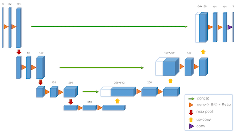
The innovation of the U-Net architecture is that it passes information from the higher-level parts of the network at the start across to the scaling-up side on the right, so structure and other information found in the initial higher levels can be used alongside information that’s passed up through the scaling-up blocks. Yay more information!

My existing architecture was basically a U-Net without the left-to-right arrows…so I thought ‘why not add them in and see what breaks?’.

I added a simple line from the first block of scaling-down filters to the last block of the scaling-up filters just to see if I’d get any benefit. And…finally, I was getting somewhere. Here’s the current architecture - the final Lambda layer is just a multiplication to bring the values of the two new channels into the CIELAB colour space for a and b:

(it turns out that Zhang and his team released a new paper in May that also includes U-Net-like additions, so we’re thinking on the same lines at least!)

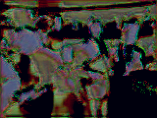
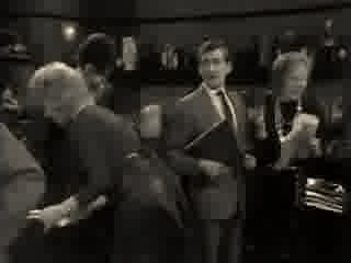
You Have Been Watching

Here’s a clip of the original b/w of ‘The Colour Problem’ side-by-side with my colourized version:

I’m not going to claim that it’s perfect. Or even wonderful. But: my partial U-Net was trained only on 5000 stills and only for 10 epochs (taking just over an hour). That it produced something akin to a fourth-generation VHS tape with no further effort on my part seems amazing.

End of Part One

Obviously, the next step is to train the net on the full dataset. This is going to require some rejigging of the training and test data, as the full 650,000 image dataset can’t fit in memory. I’ll probably be turning to bcolz for that. At that point I’ll also likely throw the code up on GitHub (after some tidying up). I’m also moving away from Amazon to a dedicated machine with a 1080Ti card, which should speed up training somewhat. I’ll probably also take a look to see if the additions in other colourization networks provide any benefit, for example adding other nets alongside the U-Net to provide local and global hints for colour. So stay tuned for part 2!